3-Phase Balanced Power Line Series Impedance and Shunt Admittance Calculator (Symmetrical Components)

This calculator derives the series impedance (Z) and shunt admittance (Y) matrices for overhead transmission lines using standard power system analysis methods. It is designed for electrical engineers and students performing load flow, short circuit, or protection coordination studies.

1. Series Impedance and Carson’s Equations

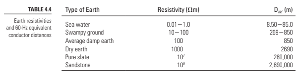
The self and mutual impedances of the conductors are calculated using Carson’s line equations (1926). This method accounts for the earth return path by modeling the ground as a fictitious return conductor located at a complex depth.

• Internal Impedance: Based on the conductor’s resistance and internal flux.
• Geometric Impedance: Derived from the physical spacing between phase conductors and their images in the earth.
• Earth Return: Adjusted based on the earth resistivity (ρ) you select. High resistivity soils (like rock) increase the zero-sequence impedance.

2. Symmetrical Components (Z₀₁₂)

Because most power system analysis is performed in the sequence domain, this tool converts the $abc$ phase impedance matrix into symmetrical components:

• Positive Sequence (Z₁): Balanced load impedance (used in load flow).
• Negative Sequence (Z₂): Equal to positive sequence for static lines (Z₁ = Z₂).
• Zero Sequence (Z₀): Critical for ground fault calculations. This value is heavily influenced by the neutral conductors and earth resistivity.

3. Shunt Admittance

The calculator also determines the capacitive susceptance of the line (charging current). It utilizes the potential coefficient matrix derived from the conductor positions and their image charges to solve for capacitance to ground and between phases.

For three-phase, balanced transmission lines.  Reports positive, negative, and zero sequence symmetrical components of line impedance.  Lines are positioned as shown below with x and y coordinates and resistivity is selected based on type of earth below the line.  Method is based on Power System Analysis and Design [1] pages 197 on.  Earth is replaced with earth return conductors as shown in the Glover textbook referencing Carson [2]

https://github.com/rsparks3/power-line-impedance-calculator/tree/main

[1] J. D. Glover, T. J. Overbye, and M. S. Sarma, Power System Analysis & Design. Boston, MA: Cengage Learning, 2017.

[2] John R. Carson, “Wave Propagation in Overhead Wires with Ground Return,” Bell System Tech. J. 5 (1926): 539–554.

System frequency:
Right of way material: Sea water Swampy ground Average damp earth Dry earth Pure slate Sandstone Custom resistivity
Ground resistivity: (ohm meter)
A Position (x, y): , (ft)
B Position (x, y): , (ft)
C Position (x, y): , (ft)
Phase conductor resistance: (ohms per mile per conductor)
Phase conductor geometric mean radius (GMR): (feet)
Phase conductor outer diameter (OD): (inches)
Phase bundle size: (cables per bundle)
Bundle spacing (if bundle size >1): (ft)

Neutral conductor count:

Neutral conductor resistance: (ohms per km per conductor)
Neutral conductor geometric mean radius (GMR): (feet)
Neutral conductor outer diameter (OD): (inches)



Series impedance:
Z₀ =
Z₁ =
Z₂ =


Shunt admittance:
Y₀ =
Y₁ =
Y₂ =

This tool calculates the sequence impedances (positive, negative, and zero) and shunt admittances for a three-phase balanced transmission line. Follow these steps to generate your parameters:

1. System Frequency: Enter your grid frequency (usually 60 Hz for North America or 50 Hz for Europe/Asia).
2. Earth Resistivity: Select the soil type for your right-of-way. This value is critical for calculating the earth return path impedance using Carson’s equations. If you have specific field data, choose "Custom resistivity."
3. Conductor Geometry: Enter the $x$ (horizontal) and $y$ (vertical height) coordinates for phases A, B, and C relative to a reference point (usually the center of the tower at ground level).
4. Conductor Properties:
   • Resistance: Input the DC or AC resistance at operating temperature (Ohms/mile).
   • GMR (Geometric Mean Radius): This is often found in conductor data sheets (e.g., for ACSR or AAC cables).
   • Bundling: If you use bundled conductors, specify the number of cables and the bundle spacing.
5. Neutrals: Add any overhead ground wires (OHGW) or neutrals. The calculator will mathematically reduce these to provide the final $3 \times 3$ phase impedance matrix before converting to symmetrical components.